# Lattice Part 2
**Describe an approximation algorithm to the Closest Vector Prolem.**
**While LLL for SVP.**
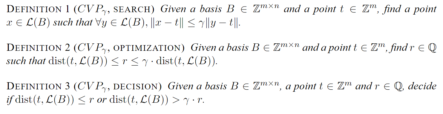
## The Closest Vector Problem
Definition :
Given a target vector $\boldsymbol{t}\in\mathbb{R}^n$ and a lattice $\mathcal{L}\subset\mathbb{R}^n$, we define
$$\operatorname{dist}(\mathcal{L},\boldsymbol{t}):=\min_{\boldsymbol{x}\in\mathcal{L}}\Vert\boldsymbol{x}-\boldsymbol{t}\Vert\:.$$
## Hardness of CVP and relationship with SVP

将 CVP 规约到 SVP 上来。
及时二者均已证明为 NP 问题,但是二者的困难程度却是迥异的。$\gamma$-SVP 要简单的多,CVP 也可视作 SVP 的非齐次形式。
一般的 SVP 工作在线性空间 $\mathcal{L}$ 上,而相对的 CVP 工作在 $\mathcal{L}$ 的一个陪集 $\mathcal{L}- t$ 上。但由于所定义短向量不包含零向量,故不可直接更换工作所在群,直接规约 CVP 到 SVP.
那么如何绕过零向量构成的难题呢?构造陪集。
### What we do in SVP
实际上这是一个存在性证明,我们回顾在处理 SVP 问题中的处理:
##### Blichfeld
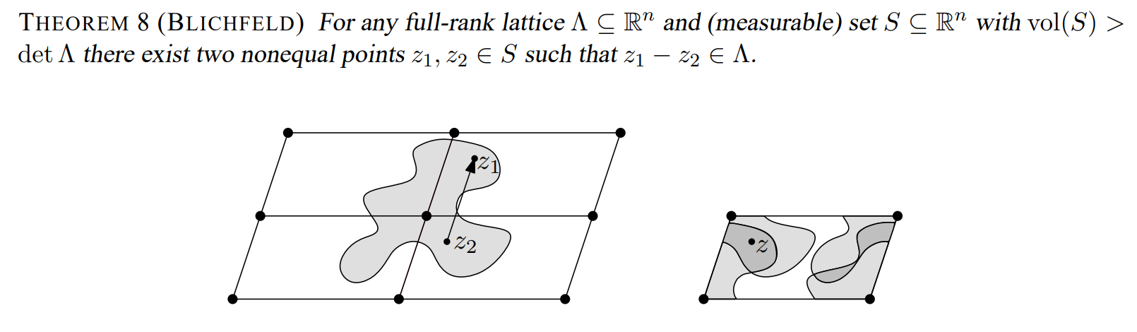
为了证明这一引理
我们介绍
##### **Fundamental Parallelepiped $\mathcal{P}(B)$**
Given the lattice basis vectors $\{b_1,b_2,\ldots,b_n\}$, the fundamental parallelepiped $\mathsf{P}(B)$ is the set of all linear combinations of these basis vectors with coefficients in the interval $[0,1)$. Mathematically, it is defined as:
$$
\mathcal{P}(B)= \set{ \sum_{i=1}^n \lambda_{i} b_{i} \mid {0} \le \lambda_{i} \lt {1} }
$$
利用这里的基本域,接着可以对整个格空间大小,以行列式为单位进行划分:

不难发现
$$
\sum_{x\in\Lambda}\operatorname{vol}(\widehat{S_x})=\sum_{x\in\Lambda}\operatorname{vol}(S_x)=\operatorname{vol}(S)>\operatorname{vol}(\mathcal{P}(B))=\det \Lambda.
$$
接下来便是优雅的鸽巢定理:

即
Since the combined volume of all $\widehat{S_x}$ is greater than the volume of $\mathcal{P}(B)$, there must be overlap among these translated regions. Therefore, there exist some $x,y \in \Lambda$ with $x \ne y$ such that $\widehat{S_x}$ and $\widehat{S_y}$ intersect:
$$
\widehat{S_x} \cup \widehat{S_y} \ne \emptyset
$$
Let $z$ be a point in this intersection. Then $z+x$ is in $S_x\subseteq S$ and $z+y$ is in $S_y\subseteq S$. The difference $(z+x)-(z+y)=x-y$ is in $\Lambda$, proving that $S$ contains at least two points whose difference is a lattice vector.
Q.E.D
##### Minkowski's Convex Body Theorem

这可以视作 Blichfeld 的推论,以为只需要注意调整系数的技巧和凸集的性质,便可证明:
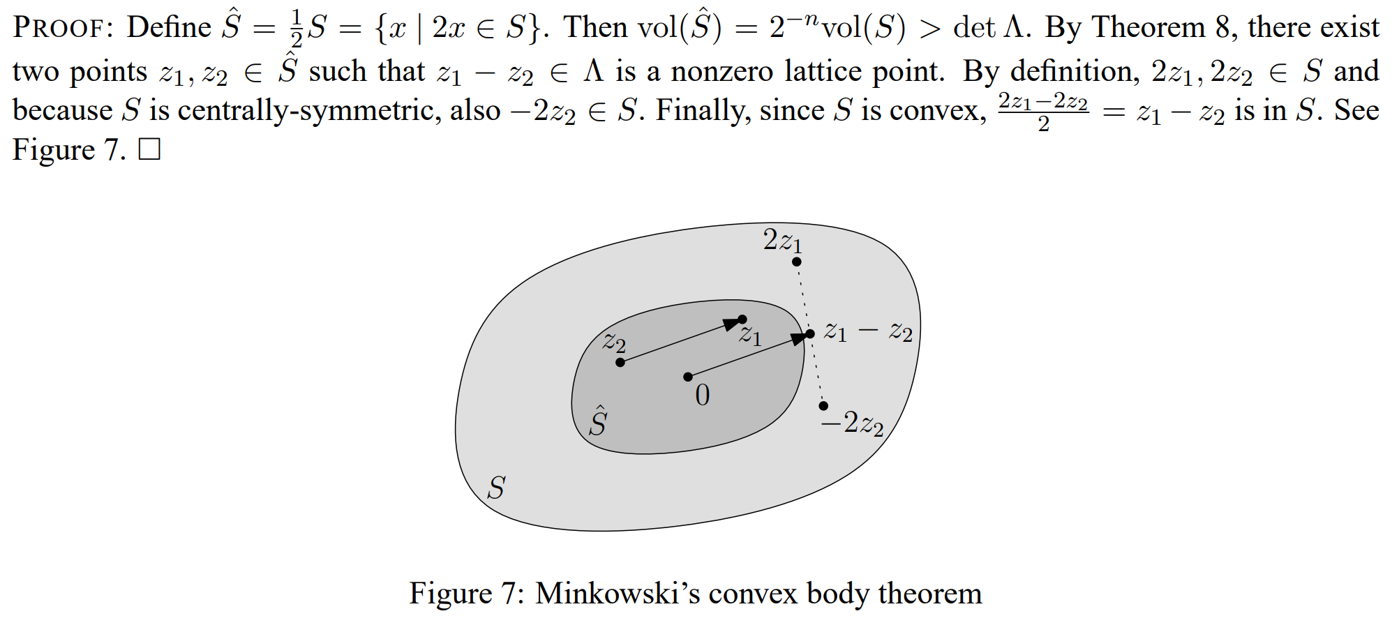
不难发现这里的系数是以集合定义来调整响应系数。利用中心对称,构造一个向量。
**综合上述思考过程,我们在坐标原点构造中心对称凸集、根据广义体积大小确定格点存在性,那么一个平凡的想法是对原有线性空间做一个划分,那么在每个划分中,可以做这样的分析来证明存在性,以此来构建近似求解 CVP 的可行性,那么在抽象代数中,对一个良好的代数结构进行划分的做法,一般的,构造陪集。**
### Reduce CVP to SVP
构造陪集的难点在于如何避开零向量的干扰。
即如何刻画一个划分,让我们的目标短向量落入其中,而零向量不在此列。技巧源于观察。观察短向量的坐标特征:
各个坐标项的至少有一个坐标为奇数(利用反证法容易证明)。具有这样特征结构的陪集,十分良好的规避了零向量的干扰。
PROOF:
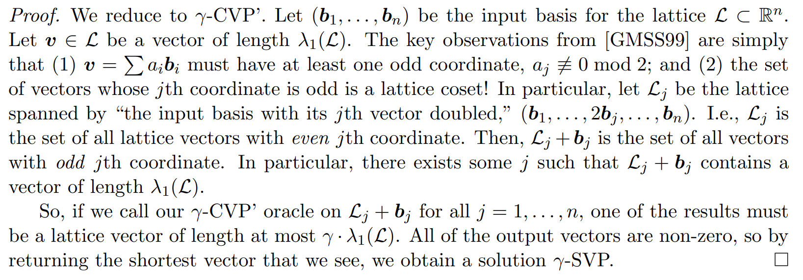
其后的处理类同 SVP 的处理。
## Babai's Algorithm
欣喜地,我们在存在性的基础上,深入学习一个近似算法。
### Pause GS in geometric
让我们留下一个基向量及其系数,来作为可以唯一确定超平面的参数
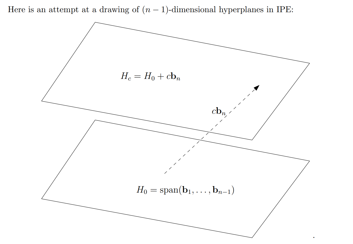
我们处理GS过程时,处理到 $b_n$ 时,便会留下一个子空间,由 $b_n$ 的线性组合决定。
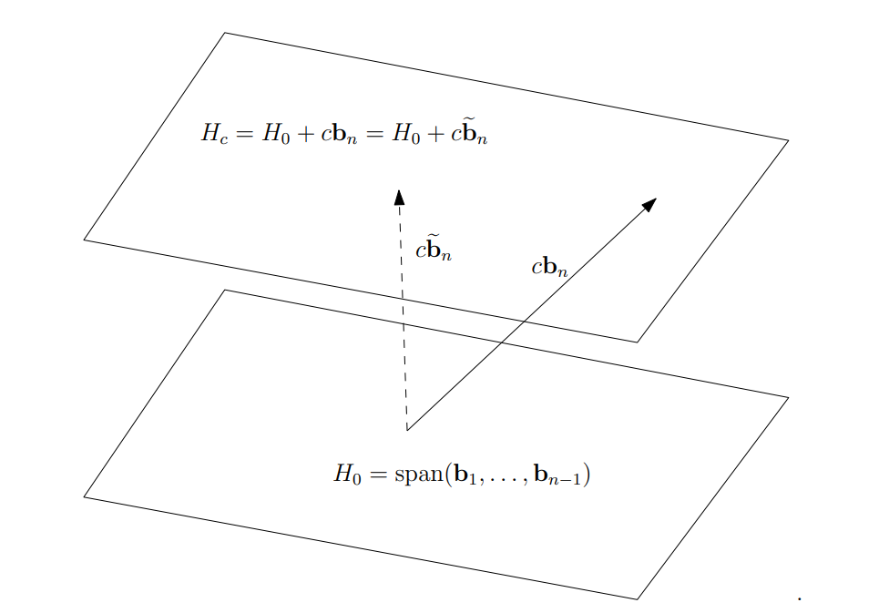
The $n$ th Gram-Schmidt vector, $\widetilde{\boldsymbol{b_n}}$ , has a very nice geometric interpretation. In particular, consider the hyperplane (i.e. affine subspace) defined by all vectors $\boldsymbol x \in\mathbb{R}^n$ (not necessarily lattice vectors) whose last coordinate is $c$ for some fixed $c$:
$$
H_{c} := \Set{ \sum_{i=1}^{n-1} a_{i} \boldsymbol{b_i} + c \boldsymbol{b_n}}
$$
Notice in particular that $H_{c} = H_{0}+c\boldsymbol{b_n}$ . But, since $\boldsymbol{b_n}$ is typically not orthogonal to $H_{0}$, the distance between $H_{0}$ and $H_{c}$ to the origin will typically not be $c \Vert \boldsymbol{b_n}\Vert$ Instead, the distance will be the length of the component of $c \boldsymbol{b_n}$ that is orthogonal to $H_{0}$ . I.e., it will be $c \Vert \widetilde{\boldsymbol{b_n}}\Vert$.
基于不同的系数 $c$ 原有格空间可以做这样的划分(以二维为例):
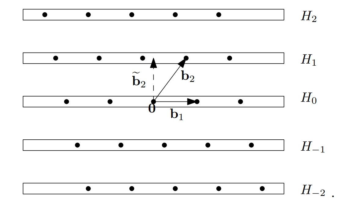
接下来用一种递归的思路,同样的可以对剩下的每个 $n-1$ 维,做同样的处理。
### Babai's nearest hyperplane algorithm
基于上述的理解模型,可以把向量 $t$ 放置于各个超平面之间:
With this picture in mind, the idea behind Babai's algorithm is quite simple. Given a target vector $\boldsymbol{t}\in\mathbb{R}^n$ and a lattice $\mathcal{L}\subset\mathbb{R}^n$ with some basis $(\boldsymbol{b_1},\ldots,\boldsymbol{b_n})$, it seems reasonable to look for a lattice vector that is close to $\boldsymbol{t}$ inside the closest lattice hyperplane to $\boldsymbol{t}$. So, Babai's $\textit{ nearest hyperplane algorithm }$ [Bab86] works by first identifying the nearest lattice hyperplane $H_c$ to $\boldsymbol{t}$. For example, Babai's algorithm would choose the hyperplane $H_{-1}$ in this example (though the closest vector to $\boldsymbol{t}$ happens to lie in $H_0$ ):
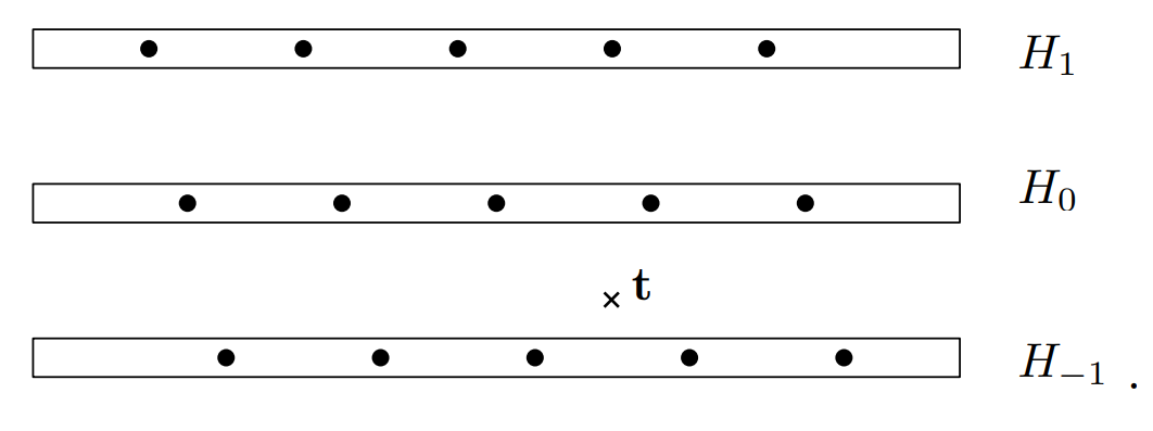
$H_c$ 包含了由 $n-1$ 个基向量张成的子格 $\mathcal{L}^{'}$ 的一个陪集 $\mathcal{L}^{'}+cb_{n}$ . 而 $\mathcal{L}^{'}+cb_{n}$ 又可继续做陪集的划分。
对 $n - i + 1$ 维 不断进行处理,则可以最终停留在一个向量上,在此前的陪集划分后,选择子空间只需不断保证欧几里得距离的最优,便可得到近似求解 CVP 问题的一个解。
### Huck Bennett suggestion
Easier to understand.
In coset $\mathcal{L} - t$ , first we rotate space so that the basis $(b_1,\dots,b_n)$ is upper triangular and looks like :
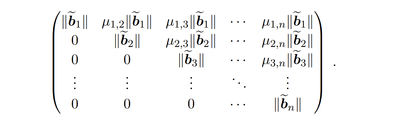
Rewrite the vector $t$ in this rotated space.
$$
\boldsymbol{t}=\begin{pmatrix}t_{1} \\\\ t_{2} \\\\ \vdots \\\\ t_{n} \end{pmatrix}
$$
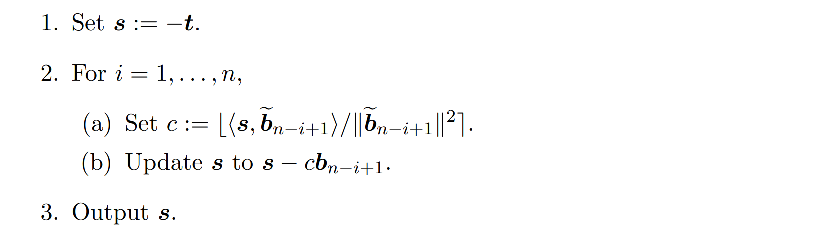
那么此前描述的陪集划分与选择的过程实际上可以重新表述为:
在给定陪集中这个寻找第 $n$ 个坐标为最小的的向量。由于每次仅处理一个基向量,故前后处理互不影响。


对于参数 $c$ 的选择依旧按照向量投影的原则,定义四舍五入的运算。那么算法最终结束时,输出 $s$ 即可。
## Analysis
### Property 1
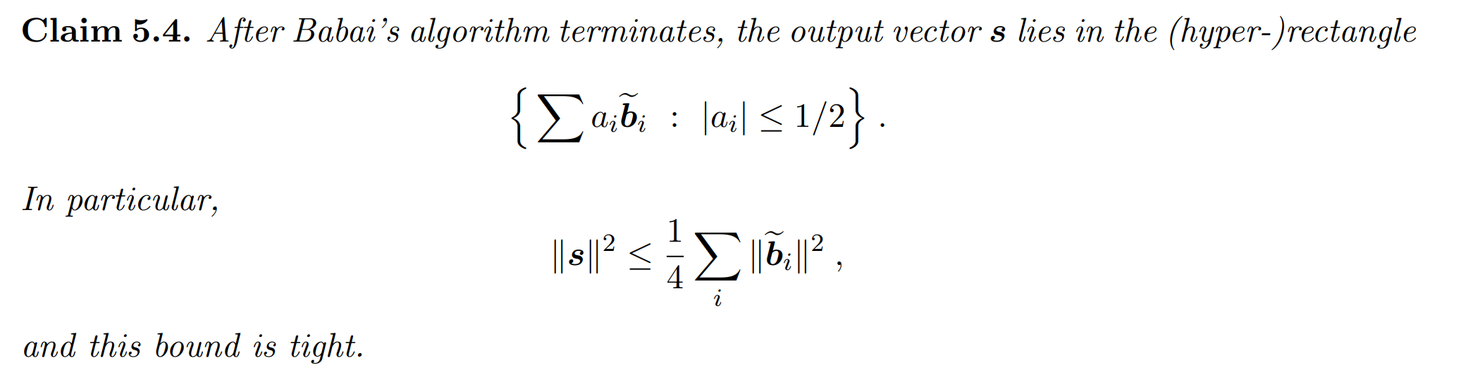
Babai Nearest Algorithm 工作在 LLL 约简基当中,故而这一性质十分显然。
GS 中可以把一个向量在基变换后重新写为:
$$
\boldsymbol{x} = \sum\frac{\langle\widetilde{\boldsymbol{b_{i}}},\boldsymbol{x}\rangle}{\Vert\widetilde{\boldsymbol{b_{i}}}\Vert^{2}}\cdot\widetilde{\boldsymbol{b_{i}}}
$$
Babai 中的系数形式为
$$
\langle\widetilde{\boldsymbol{b_{n-i+1}}},\boldsymbol{s}\rangle / \Vert \widetilde{\boldsymbol{b_{n-i+1}}}\Vert ^{2}
$$
大约在 $1/2$ 的数量级(上界),故而通过简单的不等式放缩可以证明
#### PROOF:
**Vector Decomposition Using Gram-Schmidt Vectors:**
Any vector $t\in\operatorname{span}(B)$ can be decomposed in terms of the Gram-Schmidt orthogonal basis $\{\tilde{b}_i\}:$
$$
t=\sum_{i=1}^n\alpha_i\tilde{b}_i
$$
where $\alpha_i=0$
**Approximation Quality**
Since the algorithm rounds each coefficient $\alpha_i$ to the nearest integer, the difference between $x$ and $t$ can be bounded. Specifically, for each $i$:
$$
|\alpha_i-\text{round}(\alpha_i)|\leq\frac12.
$$
Therefore, the distance between $x$ and $t$ can be expressed as a sum of these small
deviations over all Gram-Schmidt vectors:
$$
x=\sum_{i=1}^n\mathrm{round}(\alpha_i)\tilde{b}_i.
$$
Bounding the Distance:
The distance $\Vert x-t \Vert$ is thus related to the error in each dimension:
$$
x-t=\sum_{i=1}^n(\text{round}(\alpha_i)-\alpha_i)\tilde{b}_i
$$
Since |round$(\alpha_{i})-\alpha_{i}|\leq\frac12$,we have:
$$
\Vert x-t\Vert \leq\sum_{i=1}^n |\text{round}(\alpha_i)-\alpha_i| \Vert\tilde{b_i}\Vert \leq\frac{1}{2}\sum_{i=1}^{n} \Vert \tilde{b_i}\Vert.
$$
**Squared Distance Bound:**
The squared distance is then:
$$
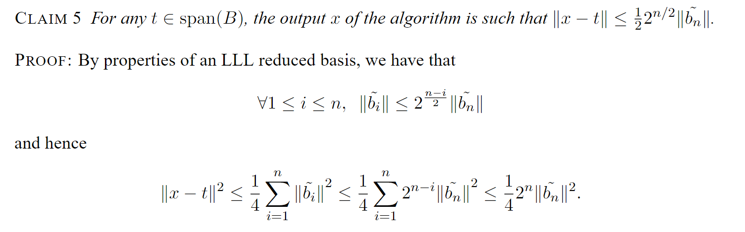
\Vert s \Vert^2 = \Vert x-t\Vert^2 \leq \left(\frac{1}{2}\sum_{i=1}^{n} \Vert \tilde{b_i} \Vert \right)^2 \leq \frac{1}{4}\sum_{i=1}^{n}\Vert \tilde{b_i}\Vert^2.
$$
The last inequality follows from the Cauchy-Schwarz inequality, which ensures that the sum of squares of the individual terms is an upper bound on the square of their sum.
In fact,
### Property 2
The output vector is determinated by the coset.

#### PROOF:
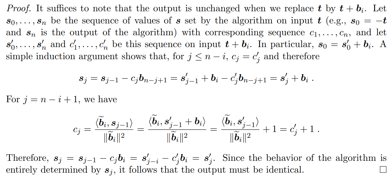
**Babai's behaviour**
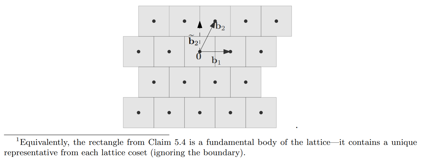
Babai's algorithm divides space into hyper-rectanges according to GS vectors.
**The output of Babai’s algorithm depends only on where the input lands modulo this tiling**
这实际上说明了 Babai 在一定范围内一定会得到想要结果,而值得深入研究的是这里的 $\gamma$-CVP 中的 $\gamma$ 是否可以找到一个上界,或这样的上界是否能够继续优化。
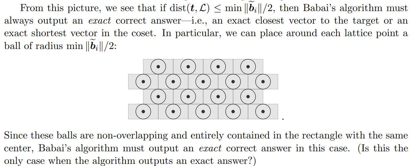
在这样的模型思考下,我们形式上可以给出一个基础的 Bound :
$$
\gamma\leq\frac{\left(\sum\Vert\widetilde{\boldsymbol{b_{i}}}\Vert^{2}\right)^{1/2}}{\min\Vert\widetilde{\boldsymbol{b_{i}}}\Vert}
$$
而这个 Bound 还有优化空间:
### Property 3

#### PROOF:
注意到:
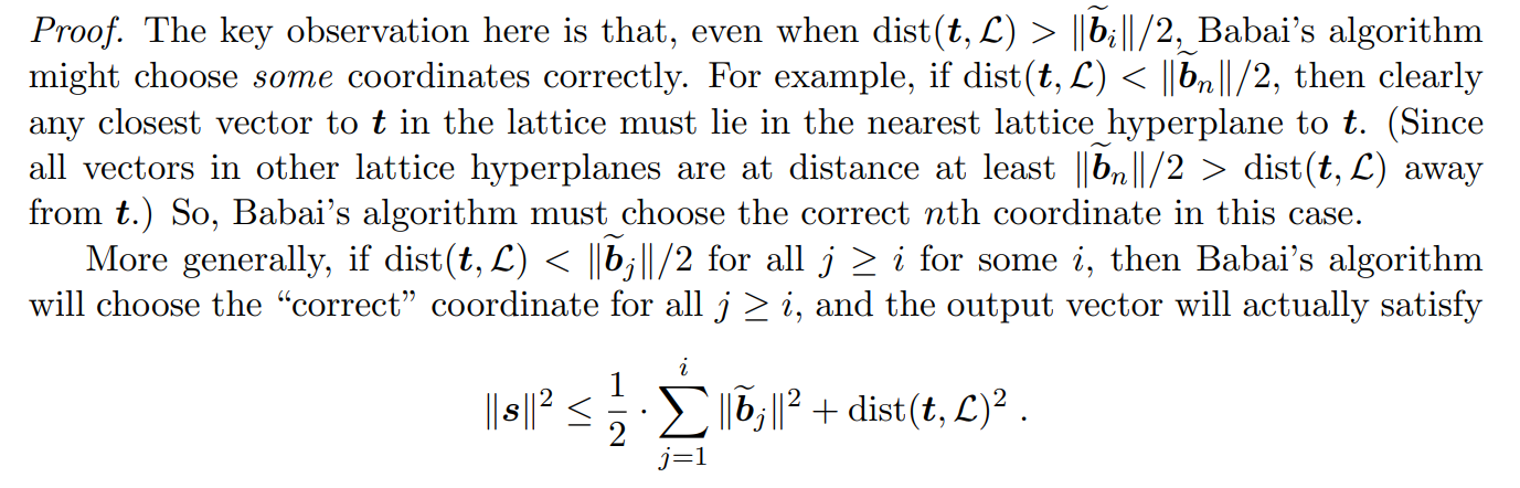
即使在$\operatorname{dist}(\boldsymbol{t},\mathcal{L})>\|\widetilde{\boldsymbol{b}}_i\|/2$的情况下,Babai 算法仍可能正确地选择某些坐标。
当 $\operatorname{dist}(\boldsymbol{t},\mathcal{L})<\|\widetilde{\boldsymbol{b}}_n\|/2$ 时,显然最近的向量在最近的格子超平面上,因为其他超平面上的向量距离 $t$ 至少 $\Vert\widetilde{\boldsymbol{b}}_n\Vert /2$, 大于$\operatorname{dist}(\boldsymbol{t},\mathcal{L})$。
所以 Babai 算法会选择正确的第 $n$ 个坐标。
更一般地,如果对于某个 $i$ , $\operatorname{dist}(\boldsymbol{t},\mathcal{L})<\Vert\widetilde{\boldsymbol{b}}_j\Vert/2$ 对所有 $j\geq i$ 成立,那么 Babai 算法将正确选择所有 $j\geq i$ 的坐标,并且输出向量满足:
$$
\|\boldsymbol{s}\|^2\leq\frac12\sum_{j=1}^i\Vert\widetilde{\boldsymbol{b}}_j\Vert^2+\operatorname{dist}(\boldsymbol{t},\mathsf{L})^2
$$
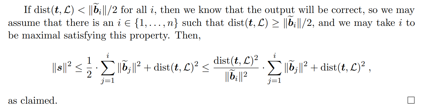
如果 $\operatorname{dist}(\boldsymbol{t},\mathcal{L})<\Vert\widetilde{\boldsymbol{b}}_i\Vert/2$ 对所有 $i$ 成立,那么我们知道输出是正确的,因此可以假设存在某个 $i\in \{1,\ldots,n\}$ 使得$\ \operatorname{dist}( \boldsymbol{t}, \mathcal{L} ) \geq \Vert \widetilde{\boldsymbol{b}} _i\Vert / 2$ , 并且可以取 $i$ 为满足此性质的最大值。
故而:
$$
\Vert\boldsymbol{s}\Vert^2\leq\frac{1}{2}\sum_{j=1}^{i}\Vert\widetilde{\boldsymbol{b_j}}\Vert^2+\operatorname{dist}(\boldsymbol{t},\mathcal{L})^2\leq\frac{\operatorname{dist}(\boldsymbol{t},\mathcal{L})^2}{\Vert\widetilde{\boldsymbol{b_i}}\Vert^2}\cdot\sum_{j=1}^{i}\Vert\widetilde{\boldsymbol{b_j}}\Vert^{2}+\operatorname{dist}(\boldsymbol{t},\mathcal{L})^2
$$
我们来看这一推导的具体细节:
PROOF
### Corollary

由 LLL 约简基的性质不难证明

Just like in the SVP case, slightly better approximation factors are known using BKZ bases (which generalize LLL bases). In particular, for any constant $C>0$, there is an efficient algorithm that solves $2^{Cn\log\log n / \log n}$-CVP
## References
- [Lattice in Cryptoanalysis](https://static.aminer.org/pdf/PDF/000/570/324/the_two_faces_of_lattices_in_cryptology.pdf)
- [Babai's Algorithm](https://www.noahsd.com/mini_lattices/05__babai.pdf)
- [CVP](https://cims.nyu.edu/~regev/teaching/lattices_fall_2004/ln/cvp.pdf)