Pae Attack
Reading: PAE
Trustworthy deep learning.
A survey on PAEs Attack.
Overview
Where it goes ?
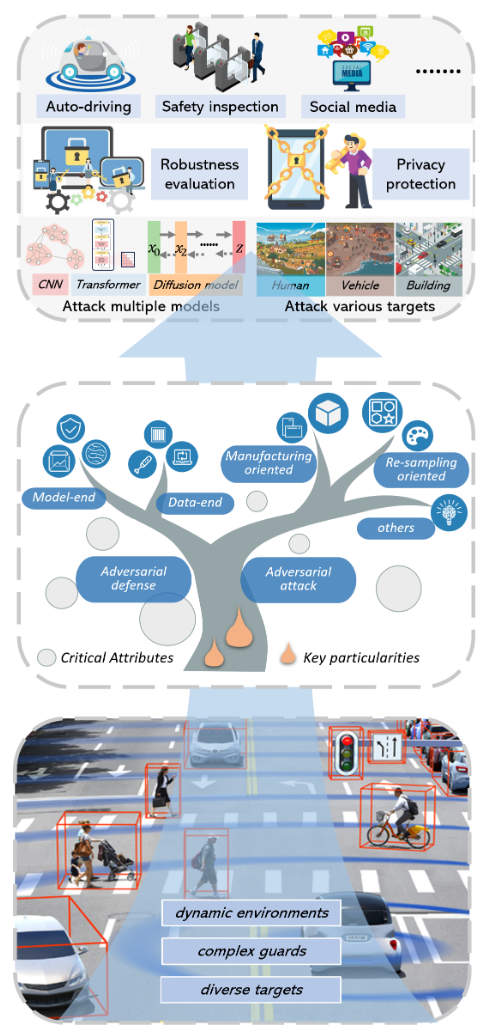
The challenges are distributed in many AI application areas.
Risk comes from application.
- CV,
- NLP
- ASR
More precisely:
auto-driving vision-based automatic check-out system vehicle classification and detection models ……
Where it from?
A critical question that what makes physical adversarial examples different from digital ones.
basically three :
- characterization
- generating strategy
- attacking ability
Substantially
- digital-physical domain gap
the physical world is a complex and open environment, where it has several dynamics such as lighting, natural noises, and diverse transformations.
On the one hand, it brings attack more various, but also harder on the other.
What we do ?
A more distinct hierarchy of physical world adversarial example generation methods
understanding of physical examples
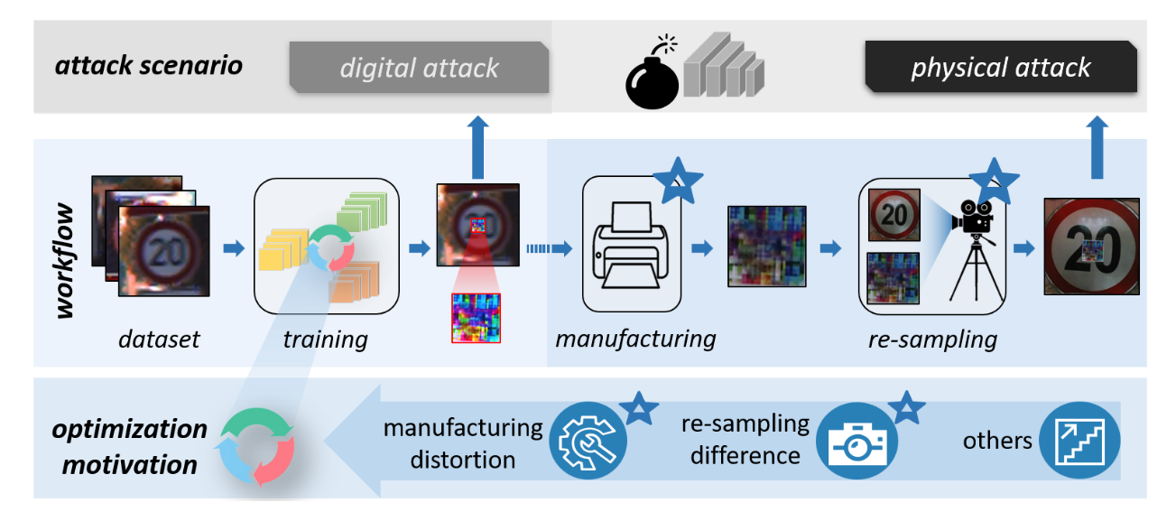
- revisit the critical particularities of physical adversarial examples under the perspective of workflow give in-depth analysis in turn to induce the typical processes that might pose a great influence on adversarial examples generation.
Three important process
- adversarial example optimization process
- adversarial example manufacturing process
- adversarial example resampling process
where the last two process are specific to the physical adversarial attacks.
Classify the PAEs:
based on the summarized typical particularities and the critical attributes, with respect to identified typical processes, according to the hundreds of physical world attack studies. Backed up by the concluded attacking particularities of the key adversarial example generation processes
Give a proposed hierarchy.
Section II - Go Deep into physical adversarial examples
overview
The digital world and physical world, divide the adversarial examples into digital kinds and physical kinds.
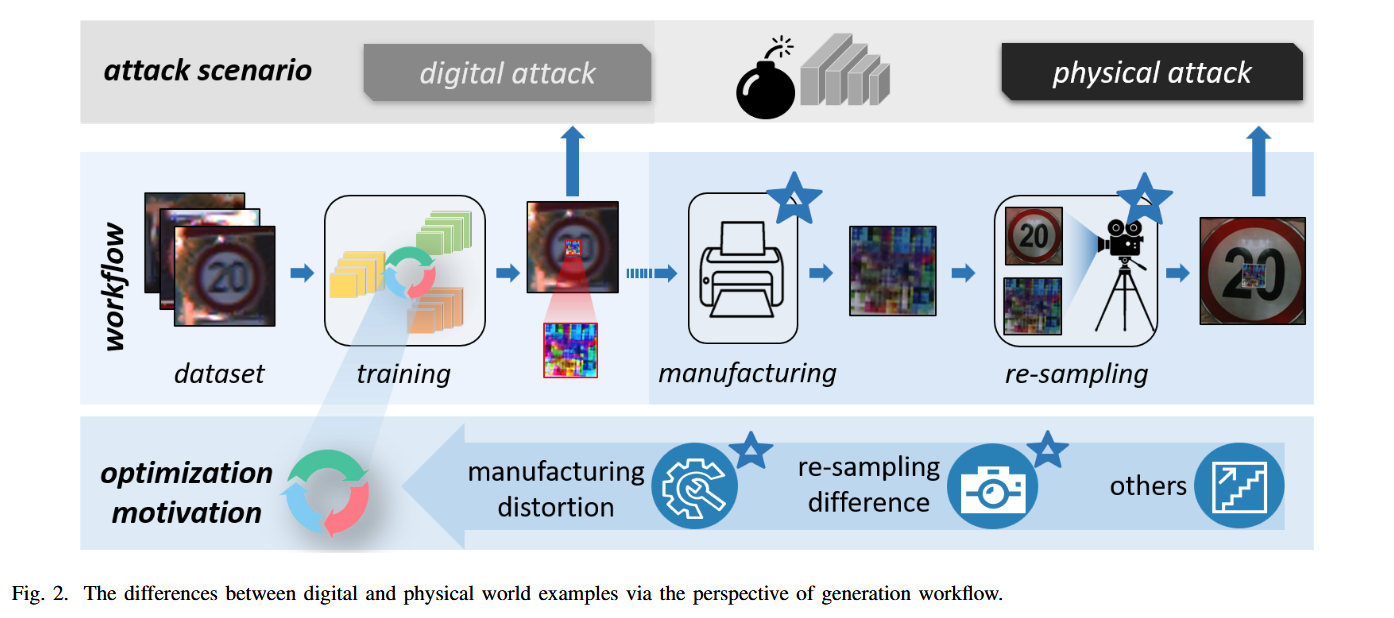
The Key Particularities among PAEs
What makes the PAEs different from the digital ones are the particular generation processes.
manufacture the digitally-trained adversarial patterns into the physical environment of existing objects, which indicates a “virtual-to-real” process.
Key:
- manufacture technique
- manufacture carrier
- sampling environment
- sampler quality
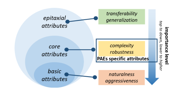
- basic attributes
- core attributes
- epitaxial attributes
Definition of PAEs
adversarial examples
$$ y^x \ne \mathcal{F}(x_{adv}^{d}),x_{adv}^{d}=x + \delta $$where $y^x$ is the ground-truth label of the input instance $x,\delta$ indicates the adversarial perturbation, and it satisfes $|\delta|<\varepsilon$ (ε is a small enough radius and bigger than 0).
Things changed in physical world.
modified definition into physical world
$$ y^x\neq\mathcal{F}(x_{adv}^p),\quad s.t.,\quad \Vert x_{adv}^p\Vert _ \aleph<\varepsilon, \\\\ x_{adv}^p=x+\mathcal{R}(\mathcal{M}(\delta),c), $$- $x_{adv}^p$ physical adversarial example
- $\mathcal{R}(\cdot)$ re-sampling function that represents the re-sampling process
- $\mathcal{M}(\cdot)$ manufacturing function that represents the manufacturing process
- $c$ a certain environment condition and comes from the real and infinite environment conditions that are denoted as $\mathbb{E},i.e.$, $c\in\mathbb{E}$
- the $|\cdot|_\aleph$ represents the evaluation metric that measures the naturalness of the PAE that input to the deployed artificial intelligence system
- $\aleph$ indicates the recognizable space of human beings to the PAEs.
where $x_{adv}^p$ is the input physical adversarial example to the deployed deep models, $\mathcal{R}(\cdot)$ is the re-sampling function that represents the re-sampling process, $\mathcal{M}(\cdot)$ is the manufacturing function that represents the manufacturing process, $c$ is a certain environment condition and comes from the real and infinite environment conditions that are denoted as $\mathbb{E},i.e.$, $c\in\mathbb{E}$, the $|\cdot|_\aleph$ represents the evaluation metric that measures the naturalness of the PAE that input to the deployed artificial intelligence system, $\aleph$ indicates the recognizable space of human beings to the PAEs.
To be brief, the $\aleph$ constraint imposed on the $\delta$ correlates to the **“suspicious” **extent of PAEs. More precisely, a very perceptible adversarial perturbation is not accepted in real scenarios.
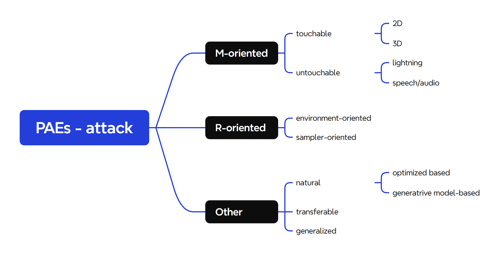
Section III .Classify PAEs
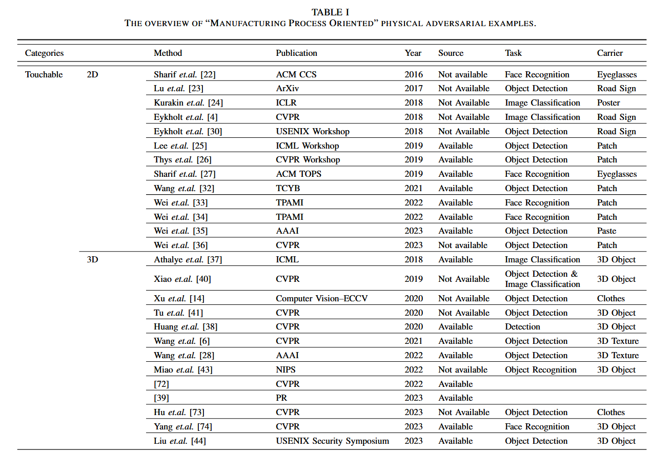
- manufacturing process-oriented ones
- re-sampling process-oriented ones
- others ( aim at naturalness, transferability )
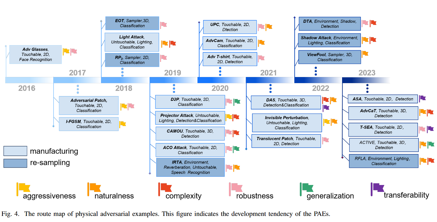
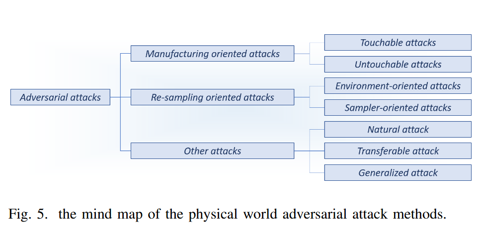
The Manufacturing Process Oriented PAEs
principles:
- material-driven
- task-driven
Our categories
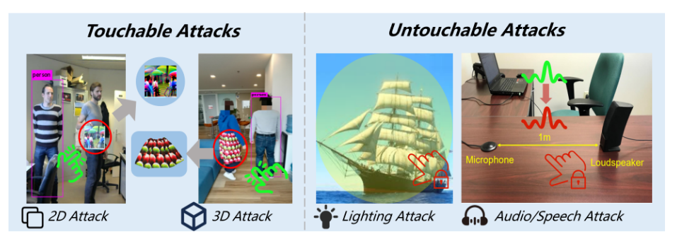
- touchable attacks
- untouchable attacks
where the former indicates that the generated adversarial examples could be touched by hands and the latter could not.
Touchable Attacks:
2D attacks
[22] M. Sharif, S. Bhagavatula, L. Bauer, and M. K. Reiter, “Accessorize to a crime: Real and stealthy attacks on state-of-the-art face recognition,” in Proceedings of the 2016 acm sigsac conference on computer and communications security, pp. 1528–1540, 2016.
smoothness and practicability
Optimize process
Total Variation Loss (using total-variation norm)
$$ L_{tv}=\sum_{i,j}\sqrt{\left(p_{i+1,j}-p_{i,j}\right)^2+\left(p_{i,j+1}-p_{i,j}\right)^2}. $$Loss function $L_{tv}$ .
practicability
Non-Printability Score
Loss function $NPS(\hat{p})$ .
$$ NPS(\hat{p})=\prod_{p\in P}|\hat{p}-p|. $$The form of this PAEs is kind of simple.
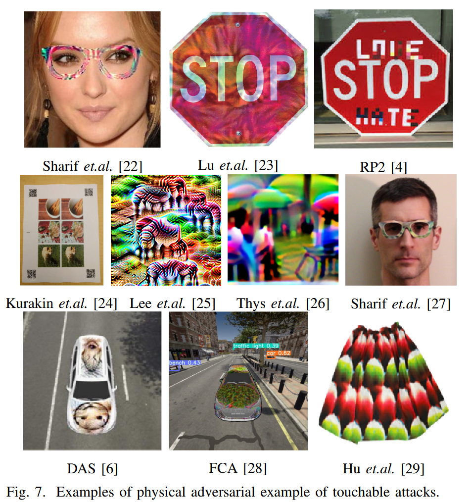
[23] J. Lu, H. Sibai, and E. Fabry, “Adversarial examples that fool detectors,” arXiv preprint arXiv:1712.02494, 2017. demonstrated a minimization procedure to create adversarial examples that fool Faster RCNN in stop sign and face detection tasks. However, due to the restrictive environmental conditions, this adversarial attack did not perform well in the physical world
[24] A. Kurakin, I. J. Goodfellow, and S. Bengio, “Adversarial examples in the physical world,” in 5th International Conference on Learning Representations, pp. 24–26, 2017.
demonstrated the possibility of crafting adversarial examples in the physical world by simply manufacturing printout adversarial examples, re-sampling them by a cellphone camera, and then feeding them into an image classification model.
[4] K. Eykholt, I. Evtimov, E. Fernandes, B. Li, A. Rahmati, C. Xiao, A. Prakash, T. Kohno, and D. Song, “Robust physical-world attacks on deep learning visual classification,” in Proceedings of the IEEE conference on computer vision and pattern recognition, pp. 1625–1634, 2018.
first generated adversarial perturbations in the physical world against road sign classifiers and proposed the Robust Physical Perturbations (RP2) algorithm. By optimizing and manufacturing white-black bock perturbation, the authors successfully attacked the traffic sign recognition model.
Robust Physical Perturbations (RP2) algorithm.
[30] D. Song, K. Eykholt, I. Evtimov, E. Fernandes, B. Li, A. Rahmati, F. Tram`er, A. Prakash, and T. Kohno, “Physical adversarial examples for object detectors,” in 12th USENIX Workshop on Offensive Technologies (WOOT 18), (Baltimore, MD), USENIX Association, Aug. 2018.
extended the RP2 algorithm to object detection tasks and manufactured colorful adversarial stop sign posters.
[25] M. Lee and Z. Kolter, “On physical adversarial patches for object detection,” arXiv preprint arXiv:1906.11897, 2019. first proposed an adversarial patch-attacking method that could successfully attack detectors without having to overlap the target objects
[26] S. Thys, W. V. Ranst, and T. Goedeme´, “Fooling automated surveillance cameras: Adversarial patches to attack person detection,” in 2019 IEEE/CVF Conference on Computer Vision and Pattern Recognition Workshops (CVPRW), pp. 49–55, 2019.
first generated physical adversarial patches against pedestrian detectors by optimizing a combination of adversarial objectness loss, TV loss, and NPS loss.
Robust Physical Perturbations (RP2) algorithm.
New Framework
previous modify adversarial examples in the perturbation process to meet additional objectives
This framework proposed a general framework to generate diverse adversarial examples. The authors utilized GANs and constructed adversarial generative nets (AGNs), which are flexible to accommodate various objectives,
e.g., inconsciousness, robustness, and scalability.
[31] T. Malzbender, D. Gelb, and H. Wolters, “Polynomial texture maps,” in Proceedings of the 28th annual conference on Computer graphics and interactive techniques, pp. 519–528, 2001.
The authors leveraged the Polynomial Texture Maps approach [31] to get eyeglasses’ RGB values under specific luminance. By using this framework, the authors constructed adversarial eyeglasses and fooled classifiers for face recognition.
SNPS
[32] D. Wang, C. Li, S. Wen, Q.-L. Han, S. Nepal, X. Zhang, and Y. Xiang, “Daedalus: Breaking nonmaximum suppression in object detection via adversarial examples,” IEEE Transactions on Cybernetics, 2021.
3D Attacks
Different 3D attack scenes.
In 2D patches is a good idea, but the spatial transformations are quite different from those of a real scene.
UPC Universal Physical Camouflage
Technique and carrior
- non-rigid or non-planar objects.
- flex or inflex surface
- changing , e. g . facing the color/texture fading
- specific shapes e. g.
- partial cover
optimization process
Let $f$ be an attack loss for misdetection, $g$ be the total-variation norm that enhances perturbations’ smoothness,
then the optimization process can be formulated as:
$$ \min \sum_i\mathbb{E_{t,t_{TPS},v}}[f(x_i,\delta)]+\lambda g(\delta) $$where $\mathbb{E}$ denotes environment conditions containing a TPS transformation $t_{TPS}\in\mathcal{T_{TPS}}$, a conventional transformation $t\in\mathcal{T}$ and a Gaussian noise $v.$ Considering the difference between flexible and rigid materials, Hu $et.al.[29]$ utilized the toroidal cropping method to manufacture arbitrary length and expandable adversarial texture.
TPS - Thin Plate Spline
Untouchable attack
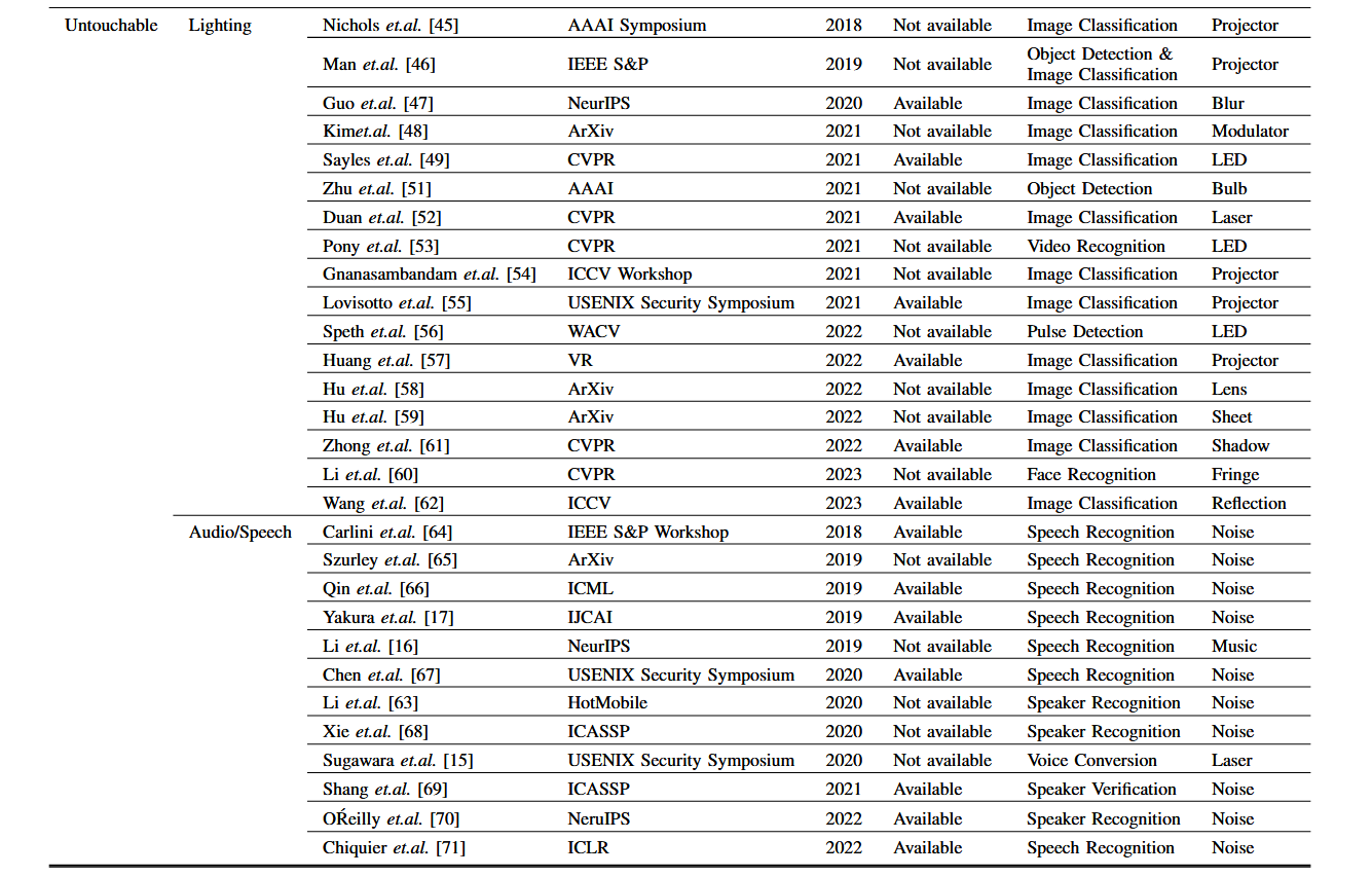
The untouchable attacks consist of lighting attacks and audio/speech attacks.
Lighting attack
-
placing a spactial light , e. g. programmable LED
-
spatial light modulator, such as SLM in front of the photographic
-
modify human non-sensitive optical parameters
-
add easily overlooked shadow, projection in special shape
All optimized.
The perturbation generation process can be formulated as follows within the context of $\mathcal{T}$ modeling environment conditions $\mathbb{E}$, which also correlates to $\mathcal{R}(\cdot)$ mentioned previously, during the re-sampling process. Let $I_{amb}$ represent the image captured under ambient light conditions, $I_{sig}$ denote the image taken under the influence of fully illuminated attacker-controlled lighting, and $g(y+\delta)$ indicate the average impact of the signal on row $y{:}$
$$ x_{adv}^p=\mathcal{T}(I_{amb})+\mathcal{T}(I_{sig})\cdot g(y+\delta). $$

Audio/Speech attacks
Speech recognition is a task to transcribe the audio/speech into text, which is then used to control the system, such as the audio assistant in mobile phones and automatic driving. Currently, some researchers develop over-the-air attacks against the deployed speech recognition system by playing the audio, impulse, and so on.
To solve the instability issues during back-propagation in the frequency domain, the author used the Discrete Fourier Transform (DFT), allowing them can perform attacks in the time domain as the symmetry properties of the DFT after the perceptual measures are extracted from the original audio.
The loss function of the manufacturing process can be summarized as:
$$ \mathcal{L}(x,\delta,y)=\mathbb{E_{t\in\mathcal{T}}}[\mathcal{L_{net}}(f(t(x+\delta)),y)+\alpha\cdot\mathcal{L_{\theta}}(x,\delta)] $$where the former term and the latter term refer to the robustness loss and imperceptibility loss, respectively.
- Voice assistants, Karplus-Strong algorithm
- voice-controllable device
- DNN-based speaker recognition system
- ……
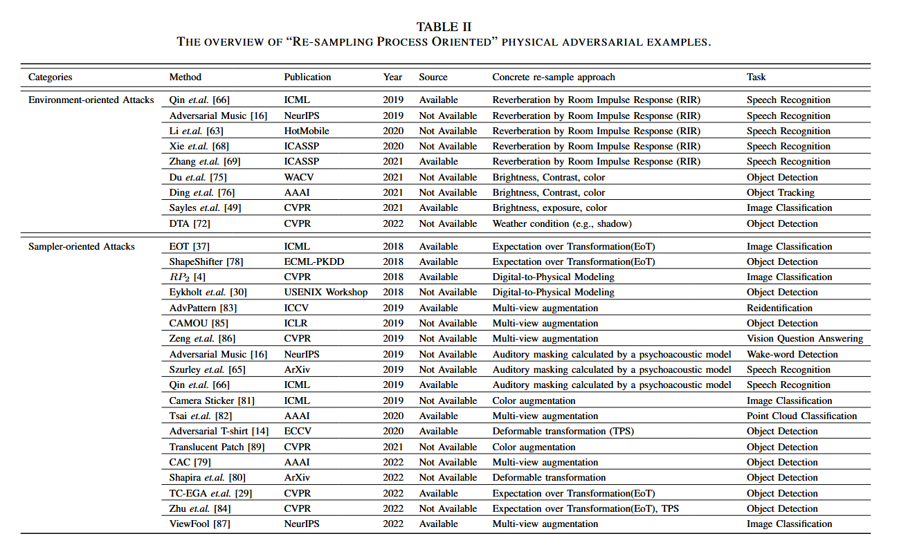
The re-sampling process-oriented ones
Shift from digital to physical with loss.
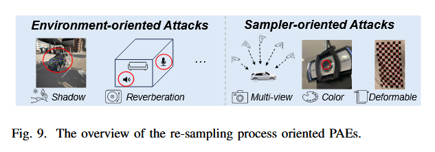
After finishing manufacturing, the physical adversarial examples will take effect by being re-sampled and input into the deployed deep models in real artificial systems. And during this process, some of the key information correlated to the adversarial characteristics inside the PAEs might be affected and cause certain attacking ability degeneration due to the imperfect re-sampling, which could be also called physical-digital domain shifts. More precisely, this kind of physical-digital shift consists of 2 types as shown in Figure 9, i.e., the environment-caused and sampler-caused, therefore motivating us to categorize the re-sampling process-oriented PAEs into environment-oriented attacks and sampler-oriented attacks.
Environment-oriented Attacks
Interference by natural factors:
- environmental lights (CV)
- environmental noises (ASR)
- ……
The physical attack performance is significantly impacted by environmental factors, such as light and weather, which motivates the researcher to take these factors into account during the optimization of PAEs. Du et.al. [75] proposed the physical adversarial attack for aerial imagery object detector, avoiding remote sensing reconnaissance. They design the tools for simulating re-sampling differences caused by atmospheric factors, including lightning, weather, and seasons. Finally, they optimize the adversarial patch by minimizing the following loss function:
$$ \mathcal{L}=\mathbb{E_{t\in\mathcal{T}}}[\max(\mathcal{F}^b(t(x_{adv}^d)))]+\lambda_1\mathcal{L_{nps}}(\delta)+\lambda_2\mathcal{L_{tv}}(\delta) $$where the first term is the adversarial loss to suppress the maximum prediction objectness score over the transformation distribution T , the second term ensures the optimized color is printable, and the last term is used to ensure the naturalness of the adversarial patch.
$$ \min \mathcal{L} $$

Import DTN
- brightness, contrast, color
- shadow
Thus, the author devised a differentiable transformation network (DTN) to learn potential physical transformations (e.g., shadow). Once DTN is trained, the author optimizes the robust adversarial texture for the vehicle via DTN.
With light attack
As we mentioned above, the adversarial LED light attack [49] also concerns the environment inside the attacking scenario. During the perturbation generation process, they propose the function T , which can be regarded as the R(·) in our definition, to model environment conditions (including viewpoint and lighting changes). In this way, they take the environmental variation during re-sampling into account to preserve the attacking ability and cross the digital-physical domain.
For physical characteristics of voice
To alleviate the potential distortion caused by the environment, a line of works [16], [63], [66], [68], [69] has adopted the room impulse response (RIP) to mimic distortion caused by the process of the speech being played and recorded, which can be expressed as:
$$ x_{adv}^d(t):r(t)=y_{adv}^p(t)*x_{adv}^d(-t), $$where the $x_{adv}^d(t)$ is the audio clip, and the $y_{adv}^p(t)$ is the corresponding estimated recorded audio clip, * denotes the convolution operation. Then, RIP $r(t)$ incorporates the generation of $\delta$ by a transform $T(x)=x*r$, which reduces the impact of distortion brought by hardware and physical signal patch, significantly improving speech physical attack robustness.
Sampler-oriented Attacks
Sampler waste adversarial information.
The case in point is sampling angles in computer vision tasks, when taking photos from different perspectives, the sampled instances might show slight differences in shape and color, e.g., affine transformation-like difference, and overexpose.
To confront the view perspective change in the physical world, Athalye et.al. [37] formulated the potential physical transformations (e.g., rotation, scale, resize) as a uniform formal that is the expectation over transformation (EOT), which is mathematically denoted as follows.
$$ \delta=\mathbb{E_{t\thicksim\mathcal{T}}}[d(t(x_{adv}^d),t(x))]. $$The above formula is designed to alleviate the data domain gap caused by transformation, enhancing the robustness of the adversarial texture.
Useful tools function imported
To keep imperceptible, adversarial after the transformation.
Specifically, they utilized the mask to constrain the perturbation to be located in the traffic sign area, and the position of the perturbation is optimized by imposing the L1 norm. The above optimization can be expressed as:
$$ > \arg \min_\delta \lambda \Vert \delta\Vert_p+\mathcal{L_{nps}}(\delta)+\mathbb{E_{x\sim X^V}} \mathcal{L} (\mathcal{F}(x+t(\delta)),y), > $$where the first term is used to bound the norm of δ for the patch’s imperceptible, the third term takes into account the transformation inside in x and applies the same transformation on δ and the $X^V$ includes the digital and physical collected training dataset.
To mimic the perspective changing in the physical world as possible
The adversarial UV is wrapped over the vehicle by changing the camera position and rendered into multi-view images. Thus, the adversarial UV texture is trained to optimize the following object function
$$ > \arg\min_\delta\mathbb{E_{x\sim X,e\sim\mathbf{E}}}[\frac1n\sum_{p_i\in P}\mathcal{L}(\mathcal{F}(x_{adv}^d,p_i),y)], > $$where E denotes the environment condition determined by the physical render, such as different viewpoints and distances; P indicates the output proposals of each image respective to the two-stage detector (e.g., Faster RCNN).
Adversarial viewpoints
Recently, Dong et.al. [87] demonstrated that there exist adversarial viewpoints, where images captured under such viewpoints are hard to recognize for DNN models. They leveraged the Neural Radiance Fields (NeRF) technique to find the adversarial viewpoints. Specifically, they find the adversarial viewpoints by solving the following problem
$$ > \max_{p(v)} \set{ \mathbb{E_{p(v)}}[\mathcal{L}(\mathcal{F}(\mathcal{G}(v)),y)]+\lambda\cdot\mathcal{H}(p(v)) } > $$where $p(v)$ denotes the adversarial viewpoints distribution $\mathcal{G}(v)$ is the render function of NeRF, which renders an image with the input viewpoints; $\mathcal{H}(p(v))=\mathbb{E_{p(v)}}[-\log(p(v))]$ is the entropy of the distribution of $p(v).$
To alleviate the influence of deformable.
Xu et.al. [14] took the Think Plate Spline (TPS) [88] method into account when optimizing the wearable adversarial patch to model the topological transformation from texture to cloth caused by body movement. Specifically, they construct the adversarial examples as following
$$ > x_{adv}^d=t_{env}(A+t(B-C+t_{color}(M_{c,i}\circ t_{TPS}(\delta+\mu v))), > $$where $t_{env}\in\mathcal{T}$ indicates the environmental brightness transform, $t_{color}$ is a regression model that learns the color covert between the digital image and its printed counterpart, $t_{TPS}$ denotes the TPS transform; $A$ is the background region expect the person, B is the person-bounded region, and C is the cloth region of the person, $v\in\mathcal{N}(0,1)$ to improve the diversity of perturbation.
Other PAE Topics
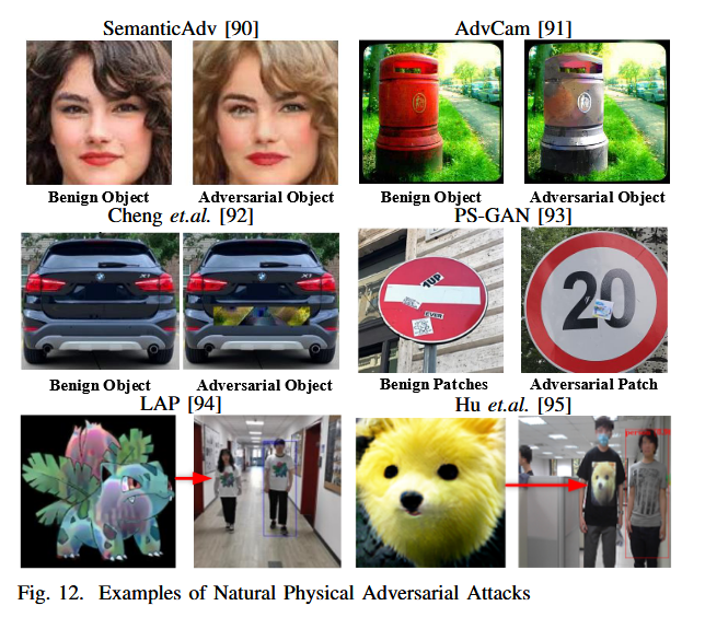
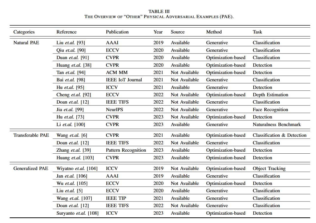
The Natural Physical Adversarial Attacks
Physical adversarial attacks often prioritize achieving high performance by ignoring the extent of modifications made to adversarial patches or camouflages. However, noticeable alterations can alert potential victims, leading to the failure of the attack. To address this, research has concentrated on creating subtle perturbations that can be deployed in real-world scenarios without detection, enabling natural physical adversarial attacks. The primary techniques employed in this area are divided into two categories:
-
Optimization-based Methods: These methods focus on refining individual adversarial examples to ensure that they are imperceptible while still effective in attacking the target model.
-
Generative Model-based Methods: In contrast to optimization-based methods, these approaches operate within the latent space of generative models that are trained on data. They leverage the learned distribution to generate adversarial examples that are both effective and difficult to detect.
The goal of this research is to develop adversarial attacks that maintain a natural appearance, increasing their stealthiness and likelihood of success when deployed against real-world systems.
Optimized-based methods
Introduce another metric function.
Initially, researchers attempted to make adversarial patches look like a particular benign patch to expose the security problems of deep learning models. A classical method applies the total-variation optimization objective mentioned in the previous sections, which improves the naturalness of the adversarial example in addition to improving the printability Duan $et.al.$ propose AdvCam [91] that minimizes $\mathcal{L_s}$, $\mathcal{L_c}$ , $\mathcal{L_{tv}}$ . The naturalness loss can be formalized as:
$$ \mathcal{L_{\text{nature}}}=\mathcal{L_s}+\mathcal{L_c}+\mathcal{L_{tv}}. $$- the style distance $\mathcal{L_s}$ between the patch and the referenced image
- the content distance $\mathcal{L_c}$ between the patch and the background
- maximizes the smoothness loss defined by the total-variation loss $\mathcal{L_{tv}}$
Generative model-based methods
In general, the generative method can be formulated as:
$$ \mathcal{L_{natural}}=\mathbb{E_{x\sim P_{real},y\sim P_{adv}}}(\mathcal{D}(x,y)), $$where $x\sim P_{real}$ are real data sampled from the training dataset, $P_{adv}$ is the distribution generated by the attack model $G_{\theta}(P_{real})$, and $\mathcal{D}(\cdot,\cdot)$ is the pre-defined (in VAE models) or adversarially learned (in GAN models) distance metric Specifically, $\tilde{\mathcal{D} } ( x, y) = - \log ( D_\theta ( x) ) - \log ( 1- D_\theta ( y) )$ in the vanilla GAN, where $D_\theta(\cdot)$ is the adversarially trained discriminator network.
The Transferable Physical Adversarial Attacks - transferability
The transferability of PAE measures whether the adversarial examples are highly aggressive across models.
Previous work on adversarial attacks in the digital world has shown that the same adversarial sample can exhibit generic attack capabilities for different deep learning models [101].
Formally, referring to Eq.(1), for the generator $\delta (x)$ trained to maximize $\mathcal{D}(y^x,\mathcal{F_{1}}(x_{adv}^p)),s.t.\Vert x_{adv}^p\Vert _{\aleph} \lt \varepsilon$, the scenario of transferable physical adversarial attacks requires that the adversarial example $\delta(x)$ be evaluated and tested on other models:
$$ \mathcal{D}(y^x,\mathcal{F_2}(x_{adv}^p)),\quad x_{adv}^p=x+\mathcal{R}(\mathcal{M}(\delta(x)),c), $$where $\mathcal{F_1}$ and $\mathcal{F_2}$ are different models.
The Generalized Physical Adversarial Attacks - robustness
The generalization ability of physical adversarial attacks, is another key to studying the limitation of the deep learning models in the real world
In general, the generalization ability over different target objects and different transformations are two important generalization problems to consider.
Formally, referring to Eq. (1), for the generator $\delta(x)$ trained to maximize $\mathcal{D}(y^x,\mathcal{F}(x_{adv}^p))$, s. t. $|x_{adv}^p|_\aleph<\varepsilon $
$$ x_{adv}^p=x+\mathcal{R}(\mathcal{M}(\delta(x)),c), x\sim P_x(x), c\sim P_c(c). $$The scenario of generalized physical adversarial attacks requires that the adversarial example $\delta(x)$ be evaluated in other data set and environment conditions, and tested in the condition of:
$$ x_{adv}^p=x+\mathcal{R}(\mathcal{M}(\delta(x)),c), x\sim P_x^{\prime}(x), c\sim P_c^{\prime}(c), $$where $P_x$ and $P_x^{\prime}$ are different data distributions, and $P_c$ and $P_c^{\prime}$ are different environmental condition distributions.
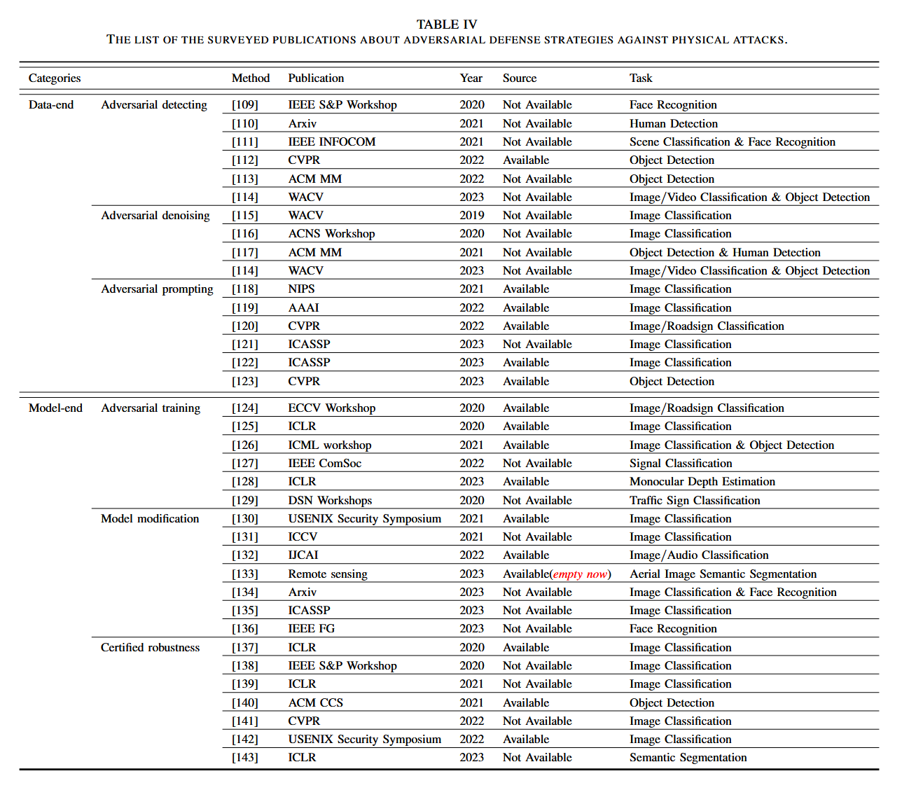
SECTION IV . CONFRONT PHYSICAL ADVERSARIAL EXAMPLES
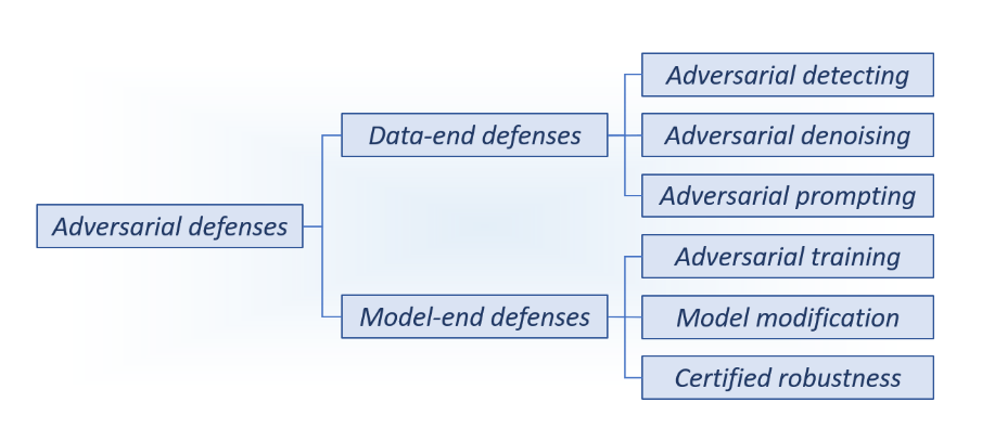
Threats makes necessity to protect intelligent applications.
Mainstream strategies
- data-end defenses
- model-end defenses
Defend against PAEs
We still take the three processes of PAEs as the starting point for thinking, considering the two standards of the data side and the model side, and considering possible defense means in various directions.
Data-end Defense Strategies
The data-end defense strategies aim to reduce the influence of adversarial perturbations, thus the sampled adversarial examples would be not allowed to mislead the deep models in deployed systems.
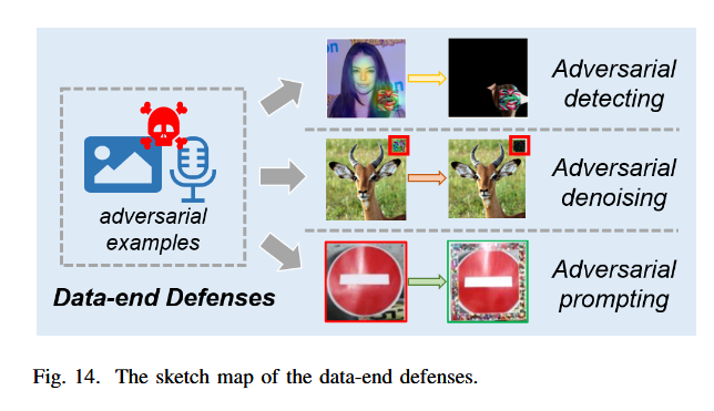
The adversarial detecting
Determining whether the input instances are adversarial. So just reject the input and evade the attack in turn.
Idea is usually simple, and the practice often has different strategies.
Summary of Adversarial Detection Methods
SentiNet (Chou et.al.)
- Detects universal adversarial patches.
- No model modifications required.
- Practical for real-world scenarios.
Ad-YOLO (Ji et.al.)
- Utilizes YOLO architecture with an added “patch” class label.
- Effective in detecting adversarial patches compared to standard YOLO.
TaintRadar (Li et.al.)
- Detects localized adversarial examples by identifying regions causing significant label variance.
- Demonstrates effectiveness in digital and physical environments.
Segmentation Approach (Liu et.al.)
- Trains a patch segmentor and performs shape completion to detect and remove adversarial patches from images.
Patch-Feature Energy-Driven Method
- Removes deep characteristics of adversarial patches to protect detection models.
Patch Zero
- Detects and nullifies adversarial patches to mitigate their influence.
Each method addresses different aspects of detecting and mitigating adversarial attacks in machine learning models.
The adversarial denoising
This kind of defense method prevents models from being fooled by adversarial attacks at the instance level, i.e., straightly removing the injected perturbation or noises inside the adversarial examples. This kind of defense could also combine with the aforementioned adversarial detecting strategy, leading to better defending ability.
A series of results from this idea:
Summary of Adversarial Defense Methods
Instance-Level Defense
- Goal: Prevent models from being fooled by removing perturbations or noises within adversarial examples.
- Combination: Can be combined with adversarial detection strategies for enhanced defense.
Local Gradient Smoothing (LGS) (Nasser et.al.)
- Targets physical attacks like Localized and Visible Adversarial Noise (LaVAN) and adversarial patches.
- Estimates regions with high probability of adversarial noise.
- Reduces gradient activity in these regions to correctly recognize adversarial examples.
Occlusion Method (McCoyd et.al.)
- Mitigates influence from adversarial patches by partially occluding the image around candidate patch locations.
- Considered a form of denoising by destroying adversarial patches through occlusion.
Adversarial Pixel Masking (APM)
- Defends against physical attacks, such as adversarial patches.
- Trains an adversarial pixel mask module to remove patches based on the generated mask.
Patch Zero
- Functions as a denoising strategy.
- Combines adversarial detection and denoising to tackle adversarial attacks.
These methods enhance the robustness of models by either directly removing adversarial perturbations or by combining detection and denoising techniques.
The adversarial prompting
Add information to offset the negative impact of adversarial perturbations, prompt what labels the models should truly predict via positive injections.
Summary of Adversarial Prompting Defense Methods
Adversarial Prompting
- Goal: Achieve defense by adding information to counteract the negative impacts of adversarial perturbations, prompting models towards correct predictions with positive injections.
Unadversarial Examples (Salman et.al.) [118]
- Generates textures with prompting ability in a 3D environment.
- Creates “robust objects” based on deep models’ input-perturbation-sensitivity.
- Provides a new approach for physical adversarial defenses.
Preemptive Robustification (Moon et.al.) [119]
- Defends against intercept-and-perturb behaviors in real scenarios.
- Utilizes a bi-level optimization scheme to discover robust perturbations that can be added to images.
Defensive Patch (Wang et.al.) [120]
- Pre-injects positive patches into instances to aid image recognition.
- Enhances prompting intensity with strong global perceptual correlations and local identifiable patterns.
- Effective against both adversarial patches and common corruptions.
Amicable Aid (Unnamed Study) [121]
- Generates visual prompting perturbations from the underlying manifold perspective.
- Provides universal improvement for classification.
Class-wise Adversarial Visual Prompting (Chen et.al.) [122]
- Addresses the non-effectiveness of universal visual prompting.
- Proposes class-specific adversarial visual prompting for enhanced effectiveness.
Angelic Patch (Si et.al.)
- Investigates visual adversarial prompting to enhance detection abilities of detectors.
These methods use various forms of positive injections and perturbations to guide models towards correct predictions, countering adversarial attacks.
Model-end Defense Strategies
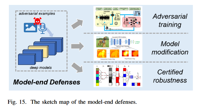
Adversarial training
Model modification
Certified robustness
